Executive assessment
This cross-sectional study contains 625 retained households from
Baoxing and Qingchuan. Application for wildlife-damage compensation is
associated with lower tolerance on several management-related measures,
but the four questionnaire outcomes do not behave as one
interchangeable scale. The safety question has little adjusted
association with application.
The rebuilt PLS model estimates a direct standardized application
path of -0.142 (95% county-stratified township-bootstrap interval
[-0.193, -0.092]). The proposed indirect association through intangible
costs is -0.025 [-0.065, 0.020]. Its interval includes zero. Neither
this result nor the institutional pathway establishes mediation. The
interaction is small and uncertain.
This supports a carefully qualified negative
association, not proof that compensation reduces tolerance or
that administrative fatigue explains it. PLS paths, ordinal log odds,
raw-score contrasts, and outcome-SD contrasts are different quantities
and must not be compared as if on the same scale.
The analysis also identifies useful secondary associations involving
prevention and agricultural dependence. These are exploratory. Every
tested specification, diagnostic, failed fit, and available result table
is retained in the analysis outputs.
1. Background, design, and hypotheses
The study asks whether compensation application is associated with
tolerance, whether intangible costs and institutional contact may link
those variables, and whether the relationships withstand reasonable
measurement and analytical choices. Mengxi’s wider dissertation concerns
cultural perceptions, policy history, and governance of human–wild-boar
conflict in China.
The Wildlife Tolerance Model motivates distinguishing conflict
exposure, tangible losses, intangible costs, perceived ecological
benefits, and tolerance. Compensation is a policy experience;
institutional contact is an observed behavior; costs and attitudes
describe lived experiences. Their conceptual roles should not be
determined by whichever path is significant.
The retained sample has 160 Baoxing interviews from August 2024 and
465 Qingchuan interviews from March–April 2025. County is therefore
confounded with survey period. This is not a before/after study. There
is no untreated-policy control group: CE0 distinguishes respondents who
report applying from those who do not, not randomly assigned policy
exposure.
The primary hypotheses concern application associations with the four
tolerance items. Direction is not required for an analysis to be
successful. Indirect paths, the application-by-cost interaction, group
differences, and secondary outcomes are explicitly exploratory. The
decisions were frozen before this rebuild, but the dataset had
previously been inspected; this is not preregistration of unseen
data.
2. Data preparation and EDA
The input workbook is preserved. All 625 IDs match between its Input
Data and Raw data sheets. The raw sheet itself contains retained
interviews and earlier derived fields, not an untouched export. The
exclusion reasons for 49 of the original 674 interviews remain
unavailable.
Tol2 and Tol3 are already reversed; Mengxi confirmed this, and the
raw Chinese responses agree. They are not reversed again. The primary
rebuild restores one missing raw Tol1 answer, missing applicant
timeliness/satisfaction answers, and missing word responses.
Payment-experience items remain undefined for non-applicants. Original
and derived values are linked in
data/derived/transformation_log.csv.
Reporting institutions are reconstructed as an increasing count.
Percentage answers above 100% are unresolved, not silently divided by
ten. The primary preference analyses exclude those values; sensitivities
retain them. Recorded area is provisionally labeled mu, without hectare
conversion. Prevention non-use is distinct from poor effectiveness among
users.
| respondents |
625.000 |
| applicants |
277.000 |
| counties |
2.000 |
| townships |
25.000 |
| villages |
178.000 |
| inside_park |
105.000 |
| missing_village |
1.000 |
| invalid_minimum_ratio |
9.000 |
| invalid_desired_ratio |
4.000 |
| damage_exceeds_area |
7.000 |
| prevention_nonusers |
83.000 |
| alpha_four |
0.338 |
| alpha_three |
0.502 |
There are 177 complete village keys plus one respondent-specific key
for the missing village, nested in 25 county–township keys. No
representativeness claim or design weights can be justified without the
sampling protocol.
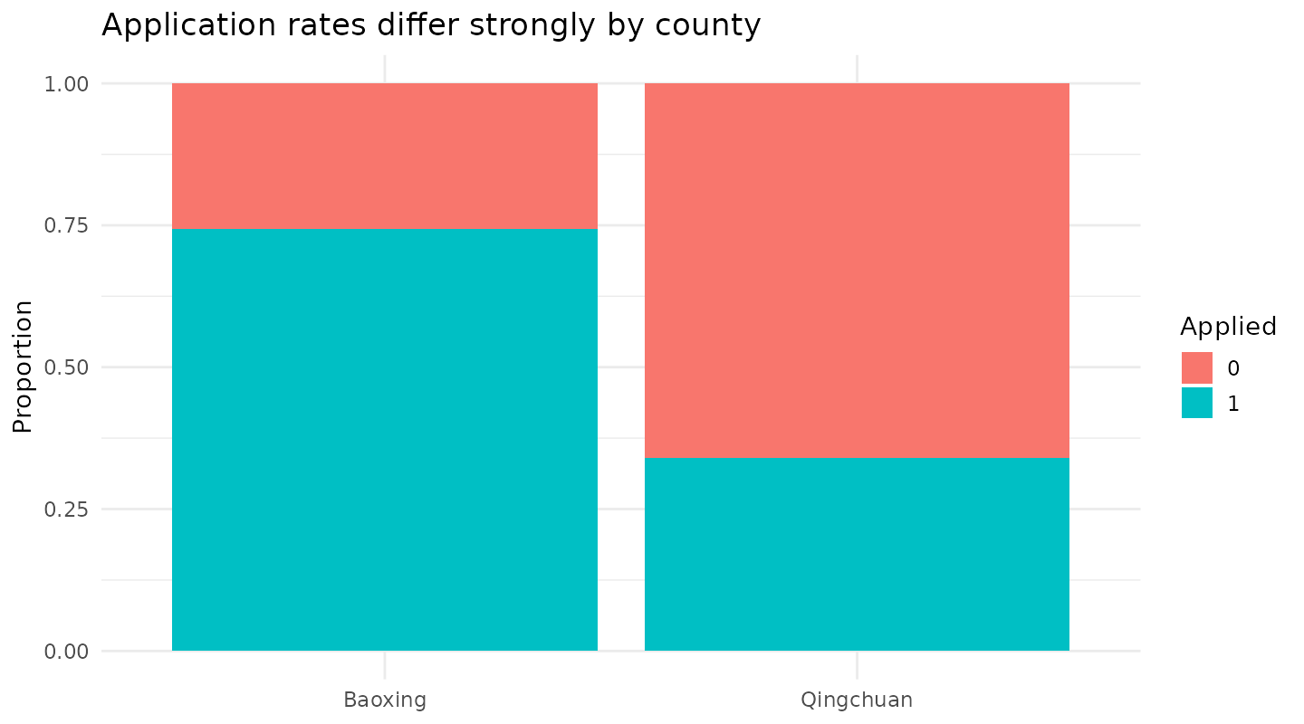
Application rates differ strongly by county (119/160 versus 158/465).
The county-adjusted results consequently answer a different comparison
from the pooled unadjusted difference. Economic variables are strongly
skewed; log1p transformations retain zeros and reduce leverage. Damage
greater than owned land is flagged, not automatically deleted, because
reference periods could differ.
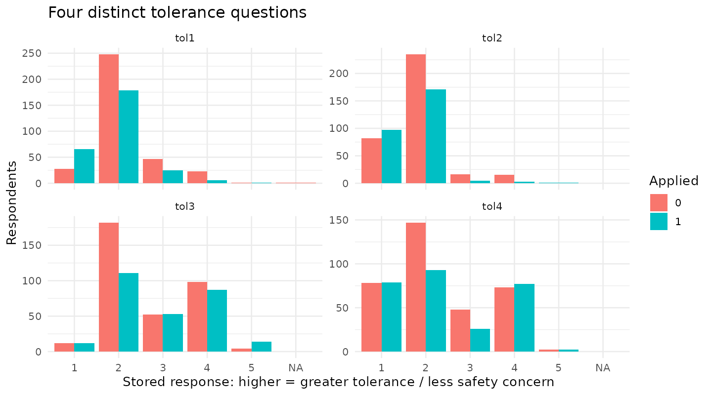
The four items concern non-lethal management, opposition to stricter
population control, absence of safety threat, and acceptance of damage.
They are substantively different. Strong floor/ceiling effects and very
sparse extreme categories matter for ordinal estimation and factor
analysis.
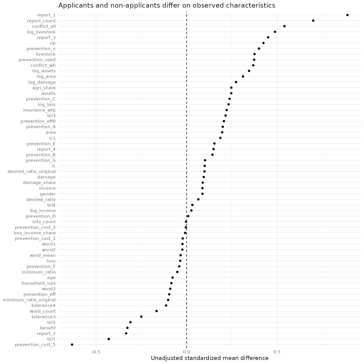
The EDA exports a numeric profile, category frequencies,
county/application/park profiles, correlations, raw-field inventory,
crop portfolio, species/seasonality/encounter frequencies, and original
Chinese-word frequencies. These full machine-readable tables accompany
this report rather than being reduced to selected significant
comparisons.
3. Measurement structure: EFA, CFA, PCA
Development and validation
A fixed village-disjoint split balances county/application cell
counts as closely as possible. Measurement exploration uses the
development partition; theory models are evaluated in the validation
partition unchanged. Full-sample estimates are then reported for
precision. Prior inspection of this dataset means this remains internal
validation, not independent confirmation.
| Baoxing |
0 |
development |
21 |
| Qingchuan |
0 |
development |
156 |
| Baoxing |
1 |
development |
60 |
| Qingchuan |
1 |
development |
79 |
| Baoxing |
0 |
validation |
20 |
| Qingchuan |
0 |
validation |
151 |
| Baoxing |
1 |
validation |
59 |
| Qingchuan |
1 |
validation |
79 |
EFA
EFA examines the four tolerance items and IC1 plus three
word-sentiment items. It uses polychoric correlations, minimum-residual
extraction, and oblimin rotation. Missing word responses are not
replaced with artificial sentiments. Correlations use available pairs;
this relies on a missingness assumption and does not solve selective
word nonresponse. There are fewer complete respondents than the pairwise
analysis count.
Sparse categories caused the initial continuity-corrected polychoric
estimator to fail. The executed analysis uses uncorrected pairwise
polychorics (correct=0, global=FALSE), with
that numerical change logged. The parallel-analysis suggestion is
examined against identification and loading structure, not accepted
mechanically.
| 1 |
0.045 |
0.810 |
0.085 |
TRUE |
316 |
238 |
4 |
| 2 |
0.029 |
0.930 |
0.051 |
FALSE |
316 |
238 |
4 |
| 3 |
0.019 |
1.004 |
0.000 |
TRUE |
316 |
238 |
4 |
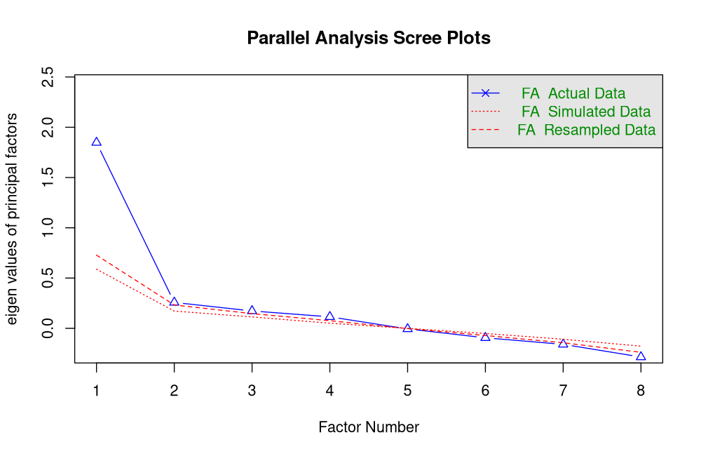
Parallel analysis suggests four factors among only eight items. A
four-factor structure with at least three indicators per factor is not
supported by this item pool, so no such CFA is manufactured. The
two-factor EFA has an ultra-Heywood solution; the three-factor
solution’s better fit does not by itself establish interpretable
constructs. This is substantive evidence against treating a neat factor
solution as guaranteed.
| tol1 |
0.524 |
0.274 |
| tol2 |
0.763 |
0.582 |
| tol3 |
0.041 |
0.002 |
| tol4 |
0.541 |
0.292 |
| ic1 |
-0.755 |
0.570 |
| word1 |
-0.218 |
0.047 |
| word2 |
-0.248 |
0.061 |
| word3 |
-0.136 |
0.019 |
| tol1 |
0.036 |
-0.035 |
0.805 |
0.606 |
| tol2 |
-0.205 |
0.150 |
0.508 |
0.504 |
| tol3 |
-0.150 |
-0.108 |
-0.021 |
0.017 |
| tol4 |
0.000 |
0.999 |
-0.002 |
0.997 |
| ic1 |
0.997 |
-0.004 |
-0.001 |
0.998 |
| word1 |
-0.056 |
-0.112 |
-0.221 |
0.060 |
| word2 |
-0.001 |
-0.212 |
-0.107 |
0.069 |
| word3 |
0.282 |
0.207 |
-0.039 |
0.074 |
CFA and discriminant validity
Ordinal CFA uses WLSMV and available-pair information. The two-factor
models separate tolerance from the proposed reflective intangible-cost
block; one alternative excludes the safety item. A one-factor model
tests empirical overlap. These are tests of measurement hypotheses, not
permission to redefine formative constructs after seeing fit.
| validation |
two_factor_four |
309 |
TRUE |
TRUE |
0.912 |
0.870 |
0.067 |
0.064 |
| validation |
two_factor_three |
309 |
TRUE |
TRUE |
0.967 |
0.947 |
0.048 |
0.051 |
| validation |
one_factor |
309 |
TRUE |
TRUE |
0.914 |
0.879 |
0.064 |
0.066 |
| full |
two_factor_four |
625 |
TRUE |
TRUE |
0.932 |
0.900 |
0.061 |
0.054 |
| full |
two_factor_three |
625 |
TRUE |
TRUE |
0.957 |
0.931 |
0.058 |
0.048 |
| full |
one_factor |
625 |
TRUE |
TRUE |
0.933 |
0.907 |
0.059 |
0.054 |
The three-item tolerance version improves validation fit, but the
combined model’s fit is not a standalone validation of a three-item
scale. Factor loadings and factor correlations matter. The full-sample
cost/tolerance factor correlation has large absolute magnitude; weak
word-item loadings and overlapping attitudinal content make a clean
separation doubtful. Factor signs are arbitrary; use loading orientation
when interpreting the correlation.
| 262 |
Tolerance |
tol1 |
0.595 |
| 263 |
Tolerance |
tol2 |
0.808 |
| 264 |
Tolerance |
tol4 |
0.454 |
| 265 |
Intangible |
ic1 |
-0.643 |
| 266 |
Intangible |
word1 |
-0.247 |
| 267 |
Intangible |
word2 |
-0.200 |
| 268 |
Intangible |
word3 |
-0.214 |
| 243 |
two_factor_four |
Tolerance |
Intangible |
0.908 |
0.683 |
1.133 |
| 305 |
two_factor_three |
Tolerance |
Intangible |
0.890 |
0.666 |
1.113 |
| Tolerance4 vs IC reflective hypothesis |
1.074 |
| Tolerance3 vs IC reflective hypothesis |
0.927 |
| Institutions vs IC (NOT applicable to formative
blocks) |
NA |
The attachment’s historical HTMT 1.112 is not reused as a current
estimate. The corrected reflective tolerance-versus-cost diagnostics
still indicate overlap. Institutional contact, however, is specified as
a formative composite of behaviors; HTMT is not an appropriate blanket
pass/fail criterion for that block. Neither merging institutional
contact with sentiment nor calling it “governance fatigue” is justified
by these questions alone.
PCA
PCA uses standardized observed items among complete cases. It
describes variance, not latent causes; it is not PLS-SEM or an
item-response model. PCA loadings and variance are supplied as an
alternative description, not selected to maximize the compensation
coefficient.
| 1 |
0.253 |
0.253 |
| 2 |
0.149 |
0.402 |
| 3 |
0.126 |
0.528 |
| 4 |
0.124 |
0.652 |
| 5 |
0.105 |
0.758 |
| 6 |
0.103 |
0.861 |
| 7 |
0.079 |
0.940 |
| 8 |
0.060 |
1.000 |
Measurement conclusion: retain the four observed
outcomes as the primary family. Use the three-item and four-item scores
transparently as secondary summaries. Treat the proposed reflective cost
factor as uncertain, and keep institutional behaviors interpretable at
item level. No single latent score should carry the whole scientific
claim.
4. Primary models and uncertainty
The primary ordinal models report application associations for all
four items, with Holm correction within each adjustment family.
Background controls are county, park residence, age, gender, education
categories, and household size. Resource adjustment adds log income,
agricultural share, log land, livestock, and assets. Explanatory models
additionally condition on simultaneous conflict, cost, benefit,
reporting, and prevention variables; these should not be described as
total causal effects.
Uncertainty clusters by township with a finite-cluster t reference.
Village clustering is a sensitivity; only two counties are available, so
county-clustered inference is not used.
| tol1 |
unadjusted |
624 |
-0.982 |
-1.409 |
-0.555 |
0.000 |
| tol1 |
background |
624 |
-0.634 |
-1.009 |
-0.259 |
0.008 |
| tol1 |
resources |
624 |
-0.668 |
-1.052 |
-0.283 |
0.006 |
| tol1 |
explanatory |
622 |
-0.469 |
-0.899 |
-0.038 |
0.083 |
| tol2 |
unadjusted |
625 |
-0.635 |
-1.039 |
-0.230 |
0.010 |
| tol2 |
background |
625 |
-0.484 |
-0.909 |
-0.060 |
0.081 |
| tol2 |
resources |
625 |
-0.561 |
-0.969 |
-0.152 |
0.027 |
| tol2 |
explanatory |
623 |
-0.517 |
-0.972 |
-0.062 |
0.083 |
| tol3 |
unadjusted |
625 |
0.396 |
0.114 |
0.677 |
0.016 |
| tol3 |
background |
625 |
0.066 |
-0.259 |
0.391 |
0.678 |
| tol3 |
resources |
625 |
0.100 |
-0.238 |
0.438 |
0.548 |
| tol3 |
explanatory |
623 |
0.225 |
-0.148 |
0.598 |
0.224 |
| tol4 |
unadjusted |
625 |
-0.002 |
-0.367 |
0.363 |
0.991 |
| tol4 |
background |
625 |
-0.304 |
-0.617 |
0.008 |
0.112 |
| tol4 |
resources |
625 |
-0.363 |
-0.644 |
-0.081 |
0.027 |
| tol4 |
explanatory |
623 |
-0.407 |
-0.721 |
-0.094 |
0.052 |
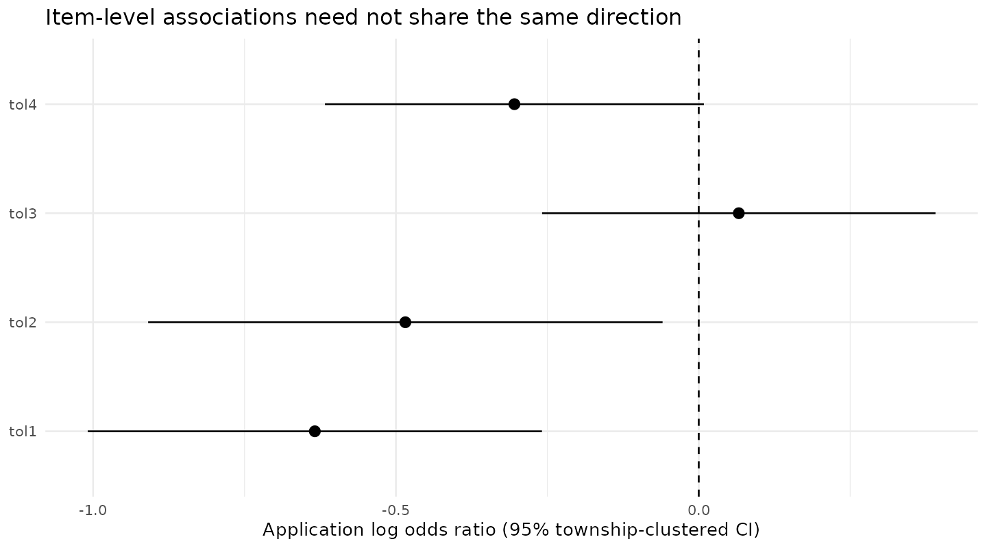
The strongest background-adjusted signal is less support for
non-lethal management among applicants. The safety item has a different
pattern. Adding resources strengthens some other item associations;
adjusting simultaneous attitudes answers another question and can
attenuate them.
Predicted category probabilities are in
ordinal_probabilities.csv. These are more interpretable
than odds ratios alone. The available partial proportional-odds
diagnostics and models are reported as sensitivity analyses, not
silently substituted to obtain favorable results.
| tol1 |
application |
3.970 |
0.265 |
| tol2 |
application |
5.234 |
0.155 |
| tol3 |
application |
8.365 |
0.039 |
| tol4 |
application |
9.265 |
0.026 |
These likelihood-ratio diagnostics are conventional individual-level
checks, not cluster-adjusted tests. Some items suggest nonparallel
application slopes. A sparse-category partial model for Tol2 has a
singular Hessian; its parameter table is retained for diagnosis but
should not be interpreted as a reliable final estimate. The ordinal
proportional-odds summaries therefore remain accompanied by category
probabilities, partial-model diagnostics, and continuous-score
sensitivity.
| tolerance3 |
unadjusted |
-0.248 |
-0.406 |
-0.090 |
0.003 |
| tolerance3 |
background |
-0.284 |
-0.452 |
-0.117 |
0.002 |
| tolerance3 |
resources |
-0.325 |
-0.483 |
-0.168 |
0.000 |
| tolerance3 |
explanatory |
-0.252 |
-0.377 |
-0.127 |
0.000 |
| tolerance4 |
unadjusted |
-0.113 |
-0.285 |
0.059 |
0.188 |
| tolerance4 |
background |
-0.232 |
-0.404 |
-0.061 |
0.010 |
| tolerance4 |
resources |
-0.264 |
-0.434 |
-0.093 |
0.004 |
| tolerance4 |
explanatory |
-0.169 |
-0.321 |
-0.017 |
0.031 |
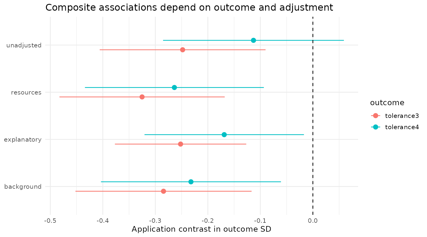
GAMs assess nonlinear age/income/land relationships in the
resource-adjusted score models. Their smooth-term and parametric tables
are saved separately; their usual model-based p-values are not
substitutes for the primary clustered inference.
Bayesian ordinal multilevel complement
Four cumulative-logit models use township random intercepts,
background controls, standardized continuous predictors, Normal(0,1)
coefficient priors, and exponential(1) random-intercept SD priors. Each
uses four chains with 1,000 warmup and 1,000 retained iterations per
chain. They make a random-effects assumption and are not a cure for
unmeasured confounding or proportional-odds misspecification.
| tol1 |
624 |
-0.626 |
-0.978 |
-0.255 |
0.000 |
TRUE |
| tol2 |
624 |
-0.462 |
-0.818 |
-0.107 |
0.005 |
TRUE |
| tol3 |
624 |
0.144 |
-0.177 |
0.474 |
0.808 |
TRUE |
| tol4 |
624 |
-0.284 |
-0.590 |
0.037 |
0.044 |
TRUE |
| tol1 |
1.005 |
1249.544 |
2062.815 |
0 |
TRUE |
| tol2 |
1.003 |
849.718 |
1655.986 |
0 |
TRUE |
| tol3 |
1.004 |
932.722 |
1765.343 |
0 |
TRUE |
| tol4 |
1.004 |
785.608 |
1023.325 |
0 |
TRUE |
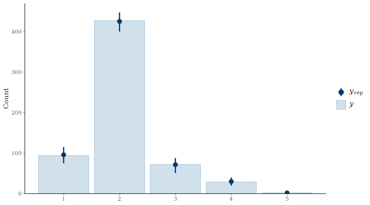
Posterior predictive figures are available for all four outcomes.
Paired posterior category contrasts use the same draws under application
0/1. Passing MCMC diagnostics establishes computational adequacy, not
causal validity or perfect model fit.
5. PLS-SEM, mechanisms, and moderation
The main PLS model contains a three-item reflective tolerance
specification; formative intangible-cost, institutional-contact, and
tangible-cost blocks; and observed application and ecological value.
Standard PLS-PM is used without disattenuation. Thus path estimates
describe standardized composite-score relationships; they are not
error-free latent causal parameters. Equal-scoring/item-level analyses
remain essential checks.
Five specifications are compared: baseline, mediation, extended
conflict/prevention, four-item tolerance, and IC1-only. All use the same
complete sample for this comparison. Formative weights, reflective
loadings, VIF, AVE, reliability, f², R², and SRMR are exported.
Interpret reflective reliability only for the reflective block; do not
use it as a requirement for formative components.
| baseline |
622 |
TRUE |
0.212 |
0.075 |
| mediation |
622 |
TRUE |
0.213 |
0.091 |
| extended |
622 |
TRUE |
0.234 |
0.074 |
| four_items |
622 |
TRUE |
0.218 |
0.091 |
| ic1_only |
622 |
TRUE |
0.187 |
0.092 |
Measurement and structural coefficients are re-estimated in every
bootstrap. Whole townships are sampled within county, preserving the
two-county design. Of 5,000 requested main-model replicates, 4999 are
usable. Failures are retained in
pls_bootstrap_replicates.csv. Both 2,000- and
5,000-replicate summaries are available for stability assessment.
| direct |
-0.142 |
-0.193 |
-0.092 |
0.000 |
4999 |
| indirect_IC |
-0.025 |
-0.065 |
0.020 |
0.248 |
4999 |
| indirect_PS |
0.024 |
-0.002 |
0.049 |
0.062 |
4999 |
| total |
-0.143 |
-0.194 |
-0.083 |
0.000 |
4999 |
| IC_to_Tol |
-0.365 |
-0.440 |
-0.260 |
0.000 |
4999 |
| PS_to_Tol |
0.072 |
-0.006 |
0.148 |
0.070 |
4999 |
| IB_to_Tol |
0.186 |
0.113 |
0.262 |
0.000 |
4999 |
| TC_to_Tol |
0.060 |
-0.069 |
0.097 |
0.223 |
4999 |
| interaction |
0.100 |
-0.074 |
0.264 |
0.254 |
4999 |
| interaction_f2 |
0.003 |
0.000 |
0.020 |
0.319 |
4999 |
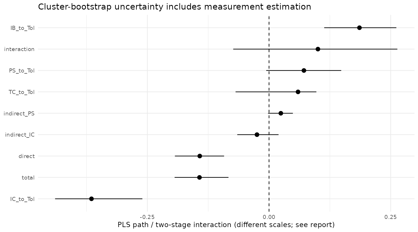
The IC and institutional indirect paths both have intervals crossing
zero. Their opposite signs nearly cancel in this specification. A
significant direct application association does not establish why it
occurs. Neither the measurement data nor temporal ordering establishes
administrative fatigue.
The two-stage interaction re-estimates PLS scores in each bootstrap,
then fits the application-by-centered-cost term. Its coefficient is
0.100 [-0.074, 0.264]; f² is approximately 0.003. It is an exploratory
small, uncertain effect. The nonnegative f² percentile interval is not a
significance test. The observed-score interaction provides a separate
common-scale comparison.
| application:ic |
0.053 |
0.047 |
-0.044 |
0.149 |
0.272 |
624 |
25 |
0.002 |
6. Multi-group analysis
Application defines the two groups; it is not included as a predictor
within either group. Measurement blocks and algorithms are the same.
MICOM’s conventional individual-permutation diagnostic uses 999
permutations; it is not a cluster-randomization test, so its p-values
are supporting diagnostics. Full output is in
logs/micom.txt.
The compositional-invariance tests do not reject, but some estimated
score correlations are low and equality of means/variances does not
generally hold. This is not proof of full invariance. Different group
standard deviations can alter standardized path coefficients.
Group path differences below use 2,000 township-cluster bootstrap
samples. Every interval includes zero. Interpret this as no
strong evidence of these group differences, not proof of
equality or support for moderation.
| IC |
0.144 |
-0.060 |
0.284 |
2000 |
| PS |
-0.031 |
-0.291 |
0.199 |
2000 |
| TC |
-0.129 |
-0.227 |
0.112 |
2000 |
| IB |
-0.034 |
-0.171 |
0.106 |
2000 |
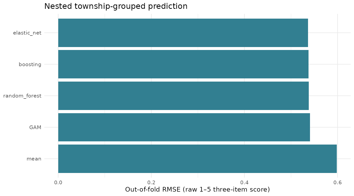
7. Prediction and cross-fitted adjustment
Prediction
Five outer township-disjoint folds evaluate prediction; three inner
township folds tune elastic net, forest, and boosting. All
imputation/scaling is learned from training rows. The score target is
the raw three-item mean, not a globally standardized latent target.
Features include directly observed attitudes, not precomputed full-data
standardized IC scores. A mean-only benchmark establishes the
baseline.
| boosting |
624 |
0.538 |
0.409 |
0.192 |
| elastic_net |
624 |
0.537 |
0.414 |
0.194 |
| GAM |
624 |
0.541 |
0.418 |
0.182 |
| mean |
624 |
0.598 |
0.452 |
-0.001 |
| random_forest |
624 |
0.538 |
0.406 |
0.190 |
| Baoxing |
mean |
160 |
0.679 |
0.000 |
| Baoxing |
elastic_net |
160 |
0.632 |
0.135 |
| Baoxing |
random_forest |
160 |
0.638 |
0.117 |
| Qingchuan |
mean |
464 |
0.567 |
0.000 |
| Qingchuan |
elastic_net |
464 |
0.524 |
0.147 |
| Qingchuan |
random_forest |
464 |
0.539 |
0.097 |
Out-of-fold performance is modest. Small differences among these
models do not prove that relationships are linear. Held-out forest
permutation importance is exported as change in MSE; it measures
predictive reliance, not causal importance. County transfer checks use
fixed hyperparameters and just two sites; they cannot establish broad
transportability.
AIPW-style adjustment
Repeated five-fold township cross-fitting estimates separate
applicant/non-applicant outcome models and application probabilities
using fixed-hyperparameter forests. Each respondent’s nuisance
predictions come from other townships. Adjustment uses background and
resource variables, not simultaneous attitudes. Propensities are bounded
at .01/.99; clipping counts, balance, and effective sample size are
exported.
| 1 |
-0.198 |
-0.300 |
-0.097 |
0.122 |
0.871 |
0 |
547.407 |
| 2 |
-0.199 |
-0.296 |
-0.101 |
0.107 |
0.880 |
0 |
532.454 |
| 3 |
-0.193 |
-0.298 |
-0.088 |
0.124 |
0.868 |
0 |
536.464 |
| 4 |
-0.195 |
-0.297 |
-0.092 |
0.102 |
0.888 |
0 |
538.327 |
| 5 |
-0.216 |
-0.322 |
-0.111 |
0.089 |
0.868 |
0 |
535.990 |
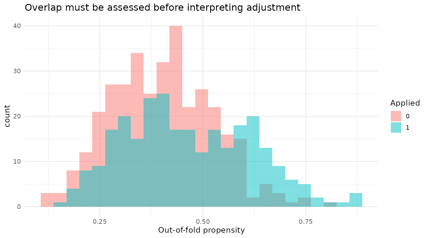
Each repetition is a sensitivity to splitting, not an independent
replication. Intervals cluster influence scores by township. These are
raw 1–5 score contrasts. Their interpretation as treatment effects would
require unverified consistency, exchangeability, temporal ordering, and
overlap assumptions. No causal claim is made.
8. Broader exploratory contribution
| application_selection |
625 |
0.087 |
-0.031 |
0.205 |
0.301 |
| applicant_timeliness |
275 |
0.013 |
-0.097 |
0.123 |
0.861 |
| applicant_satisfaction |
276 |
-0.018 |
-0.103 |
0.066 |
0.746 |
| applicant_both_experiences |
274 |
-0.043 |
-0.178 |
0.091 |
0.746 |
| livelihood_dependence |
624 |
0.250 |
0.103 |
0.398 |
0.031 |
| damage_burden |
624 |
-0.171 |
-0.349 |
0.008 |
0.169 |
| income_loss_burden |
605 |
-0.004 |
-0.022 |
0.013 |
0.746 |
| prevention_adoption |
625 |
1.134 |
0.358 |
1.910 |
0.035 |
| prevention_effectiveness_users |
541 |
0.132 |
0.041 |
0.222 |
0.035 |
| insurance_positive_wtp |
625 |
0.524 |
0.067 |
0.981 |
0.090 |
| insurance_positive_amount |
492 |
0.082 |
-0.135 |
0.298 |
0.746 |
| minimum_ratio_validated |
616 |
0.000 |
-0.032 |
0.033 |
0.986 |
| minimum_ratio_retain_flagged |
625 |
-0.107 |
-0.246 |
0.033 |
0.301 |
| desired_ratio_validated |
621 |
0.013 |
-0.039 |
0.064 |
0.746 |
| desired_ratio_retain_flagged |
625 |
0.015 |
-0.040 |
0.071 |
0.746 |
| reporting_contacts |
622 |
0.130 |
0.025 |
0.236 |
0.074 |
| information_channels |
622 |
-0.047 |
-0.138 |
0.044 |
0.562 |
The broad secondary family receives Benjamini–Hochberg adjustment.
These estimates involve different outcomes/scales and must not be ranked
by coefficient size. Notable avenues include agricultural dependence,
prevention adoption, and effectiveness among users. Applicant
satisfaction/timeliness associations are imprecise and do not establish
the proposed mechanisms.
| applicants |
277 |
| numeric_unambiguous_payouts_applicants |
161 |
| median_available_payout |
60 |
| timeliness_observed |
275 |
| satisfaction_observed |
276 |
| zero_income |
19 |
| loss_income_undefined |
19 |
| A |
248 |
377 |
2.153 |
55 |
500 |
| B |
391 |
234 |
2.026 |
115 |
200 |
| C |
339 |
286 |
2.909 |
3 |
0 |
| D |
56 |
569 |
2.893 |
0 |
NA |
| E |
147 |
478 |
2.340 |
14 |
0 |
| F |
10 |
615 |
1.100 |
0 |
NA |
| G |
6 |
619 |
1.333 |
0 |
NA |
Prevention letters follow the raw coded fields, whose Chinese
descriptions are retained in the full table. Monetary cost nonresponse
is common. We do not calculate causal benefit–cost rankings from these
incomplete, self-selected responses. Payout amounts are accepted only
when the text is an unambiguous numeric response in exactly one amount
field; payout/loss ratios are withheld until reference periods are
confirmed.
The raw questionnaire supports crop-specific losses, seasonal
descriptions, encounters, species, and original-word frequencies. Their
complete tables are included. Seasonality is recalled timing, not a
repeated-measures panel. Word-frequency counts do not establish
validated psychological themes; human Chinese-language interpretation
remains necessary.
9. Robustness, vibration of effects, and selective-reporting
risk
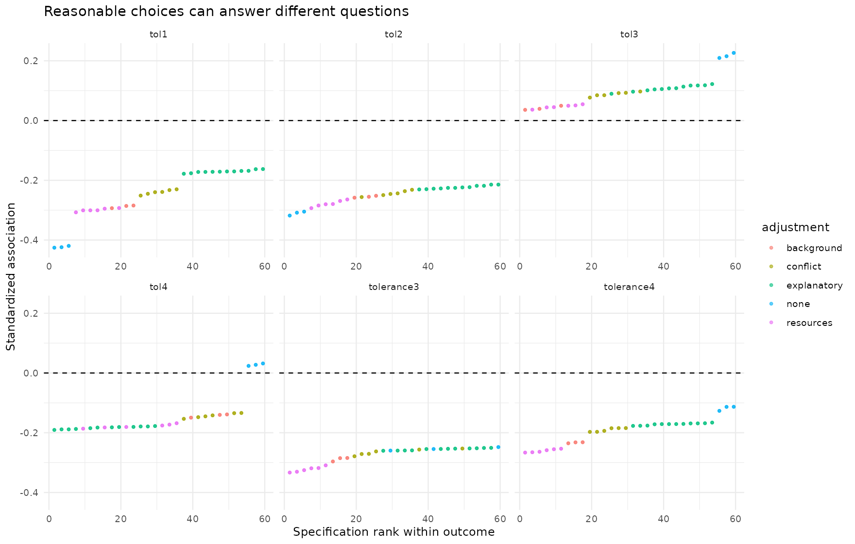
The specification curve crosses prespecified outcomes, adjustment
families, raw/log economic predictors,
extreme-loss/reporting-contradiction handling, and complete-case versus
median/mode covariate sensitivity. Identical model inputs are
deduplicated before estimation. Township/village uncertainty variants
are retained explicitly. Outcomes are displayed separately because they
answer different questions.
Single median/mode imputation is only a limited sensitivity for the
few incidental covariate gaps; it is not multiple imputation and does
not account for imputation uncertainty. Structural payment nonresponse
and missing words are not imputed.
| tol1 |
background |
6 |
-0.293 |
-0.286 |
-0.285 |
1 |
| tol2 |
background |
6 |
-0.258 |
-0.255 |
-0.252 |
1 |
| tol3 |
background |
6 |
0.036 |
0.039 |
0.049 |
0 |
| tol4 |
background |
6 |
-0.149 |
-0.140 |
-0.139 |
1 |
| tolerance3 |
background |
6 |
-0.296 |
-0.285 |
-0.284 |
1 |
| tolerance4 |
background |
6 |
-0.235 |
-0.232 |
-0.232 |
1 |
| tol1 |
conflict |
12 |
-0.251 |
-0.239 |
-0.230 |
1 |
| tol2 |
conflict |
12 |
-0.256 |
-0.245 |
-0.232 |
1 |
| tol3 |
conflict |
12 |
0.077 |
0.088 |
0.097 |
0 |
| tol4 |
conflict |
12 |
-0.153 |
-0.144 |
-0.134 |
1 |
| tolerance3 |
conflict |
12 |
-0.279 |
-0.267 |
-0.253 |
1 |
| tolerance4 |
conflict |
12 |
-0.197 |
-0.189 |
-0.184 |
1 |
| tol1 |
explanatory |
24 |
-0.178 |
-0.171 |
-0.162 |
1 |
| tol2 |
explanatory |
24 |
-0.231 |
-0.225 |
-0.214 |
1 |
| tol3 |
explanatory |
24 |
0.090 |
0.108 |
0.122 |
0 |
| tol4 |
explanatory |
24 |
-0.191 |
-0.182 |
-0.178 |
1 |
| tolerance3 |
explanatory |
24 |
-0.260 |
-0.254 |
-0.251 |
1 |
| tolerance4 |
explanatory |
24 |
-0.177 |
-0.171 |
-0.166 |
1 |
| tol1 |
none |
6 |
-0.426 |
-0.424 |
-0.420 |
1 |
| tol2 |
none |
6 |
-0.318 |
-0.308 |
-0.305 |
1 |
| tol3 |
none |
6 |
0.209 |
0.215 |
0.226 |
0 |
| tol4 |
none |
6 |
0.024 |
0.027 |
0.032 |
0 |
| tolerance3 |
none |
6 |
-0.260 |
-0.255 |
-0.248 |
1 |
| tolerance4 |
none |
6 |
-0.127 |
-0.113 |
-0.113 |
1 |
| tol1 |
resources |
12 |
-0.307 |
-0.301 |
-0.293 |
1 |
| tol2 |
resources |
12 |
-0.293 |
-0.280 |
-0.264 |
1 |
| tol3 |
resources |
12 |
0.036 |
0.047 |
0.055 |
0 |
| tol4 |
resources |
12 |
-0.186 |
-0.178 |
-0.168 |
1 |
| tolerance3 |
resources |
12 |
-0.333 |
-0.322 |
-0.309 |
1 |
| tolerance4 |
resources |
12 |
-0.266 |
-0.261 |
-0.253 |
1 |
These curves describe analytical sensitivity. They cannot establish
that p-hacking never occurred, and the fraction negative/significant is
not a posterior probability or an independent-replication count.
Historical incorrect reverse coding is excluded from the set of
reasonable primary specifications.
| Leave-one-township-out application contrast |
-0.353 |
-0.289 |
| Baoxing |
-0.381 |
-0.786 |
0.024 |
160 |
5 |
| Qingchuan |
-0.302 |
-0.494 |
-0.111 |
464 |
20 |
The omitted-confounding grid benchmarks how a hypothetical omitted
variable could move the resource-adjusted linear estimate toward zero.
It uses partial-R² values for outcome and application residuals. This is
a point-estimate bias calculation, not a cluster-adjusted confidence
bound, and no particular strength is asserted to be realistic.
| 0.00 |
0.00 |
0.000 |
-0.195 |
-0.195 |
| 0.01 |
0.01 |
0.013 |
-0.195 |
-0.182 |
| 0.03 |
0.03 |
0.039 |
-0.195 |
-0.155 |
| 0.05 |
0.05 |
0.066 |
-0.195 |
-0.129 |
| 0.10 |
0.10 |
0.136 |
-0.195 |
-0.059 |
| 0.20 |
0.20 |
0.288 |
-0.195 |
0.093 |
10. Answers to the Exploratory Contribution
| Do the indicators form the expected constructs? |
Not cleanly. Sparse categories, weak word loadings, factor overlap,
and weak safety-item coherence challenge a single tidy measurement
model. |
| Remove, reassign, or merge indicators? |
Present observed outcomes as primary. Three-item tolerance is a
transparent sensitivity. No automated significance-driven deletion or
institution–sentiment merger. |
| Is policy support distinct from intangible costs? |
The institutional indicators measure contact/information behavior,
not reflective fatigue. Evaluate their interpretation and formative
construction before applying HTMT. |
| Are the proposed structural models defensible? |
They are useful exploratory association models. Compare baseline and
extended versions; contemporaneous data do not identify path
direction. |
| Does the indirect cost pathway hold? |
Its cluster-bootstrap interval includes zero in the rebuilt main
model. Do not claim demonstrated mediation. |
| Does the interaction matter? |
Its f² is small and its interval crosses zero. Retain in
exploratory/supplementary results, not as the central mechanism. |
| What does nonsignificant MGA mean? |
No strong evidence of differences on the tested paths, conditional
on measurement comparability. Not equivalence. |
| Is the paradox robust? |
Several negative management-related associations persist.
Conclusions depend on the tolerance dimension and adjustment; the safety
item differs. “Negative association among applicants” is more precise
than “policy failure.” |
| Has p-hacking been ruled out? |
No statistical test can certify that here. The decision register,
complete outputs, honest validation, and deduplicated multiverse reduce
selective-reporting risk. |
11. Limitations and implementation boundaries
- Cross-sectional, nonrandom application; no verified treatment
timing, payment receipt, or pre-policy baseline.
- Two counties observed in different periods; unknown
sampling/exclusion processes limit generalizability.
- Limited reflective measurement, overlapping attitudes, word
nonresponse, and incomplete raw cleaning provenance.
- Ordinal proportional-odds assumptions are imperfect for some items;
sparse alternatives can be unstable.
- Conventional CFA/MICOM diagnostics do not fully model the sampling
design; clustered structural/association checks are complementary.
- Exploratory analyses reuse this finite sample. Internal splits and
cross-fitting do not turn the dataset into independent confirmatory
evidence.
- Some planned extensions require information not in the workbook:
validated thematic coding, comparable payout/loss periods, sampling
weights, and causal policy identification. They are explicitly
withheld.
No outcome was selected because it produced the desired sign.
Numerical warnings and earlier failed attempts remain in the event log.
The archived legacy results are not overwritten. This release is
suitable for methodological discussion; the report can be amended
transparently after the presentation and Mengxi’s clarifications.
12. Reproduction and references
From the project root:
Rscript run_project.R --restore
Rscript run_project.R
Rscript run_project.R --render
Rscript run_project.R --verify
renv.lock records packages;
run_manifest.json records source/data hashes and session
information. The targets graph rebuilds changed stages. Source data,
code, derived tables, and figures remain distinct. The PowerPoint and
speaker notes read these same saved results.
Methodological references: